
Automatic Relevance Determination Regression for Time Series Forecasting
Unconventional Machine Learning Models for Conventional Forecasting

Time-series models are often given a large collection of possible inputs. A forecasting system may receive recent observations, older observations, rolling averages, volatility estimates, calendar information, and related external variables. Some of these inputs may contain useful information. Others may be redundant, unstable, or entirely irrelevant.
This creates a practical problem. Adding more inputs gives the model more information to consider, but it also gives the model more opportunities to learn accidental patterns from the training data. A model may appear accurate during development because it has adapted to noise that will never occur in the same form again.
Automatic Relevance Determination Regression, available in scikit-learn as ARDRegression, approaches this problem by allowing the model to reduce the influence of inputs that do not appear consistently useful.
Rather than treating every input as equally deserving of attention, the model repeatedly evaluates how much each one contributes. Inputs that provide little dependable value are weakened. Some are effectively removed. The remaining inputs receive greater responsibility for the final prediction.
This makes ARDRegression particularly interesting for time-series research, where researchers frequently create dozens or hundreds of lagged observations without knowing which parts of the past are genuinely relevant.
The central idea in plain language
Imagine asking a group of witnesses to describe what happened during an event.
Some witnesses saw the event clearly. Some only saw part of it. Several heard the story from somebody else. Others were present but paid no attention. One person confidently remembers details that never happened.
A conventional model listens to everyone and tries to determine how much weight to give each account. This can work when the useful witnesses are obvious and the unreliable ones are harmless. It becomes less dependable when many witnesses repeat similar stories or when random details happen to fit the available evidence.
ARDRegression behaves more cautiously. It begins by allowing every witness to contribute. It then repeatedly checks whether each contribution appears necessary. Witnesses whose information does not add dependable value gradually lose influence. Some are ignored almost completely.
In a time-series setting, the witnesses are usually past observations.
A model might receive the value from one period ago, two periods ago, three periods ago, and so on. It may also receive rolling statistics or external variables. ARDRegression tries to determine which of these historical clues deserve to remain active.
Scikit-learn implements this as an iterative model. During training, it repeatedly updates the estimated influence of each input and can remove inputs that its internal relevance test considers too weak. The official documentation describes this removal process through the model’s threshold_lambda setting.
The practical result is a model that can begin with a broad set of candidate inputs and finish with a narrower set of active influences.
ARDRegression does not understand time automatically
ARDRegression is a general regression algorithm. It has no built-in understanding of sequence, chronology, cycles, or market history.
If it receives a column of values, it does not automatically know that one row occurred after another. It sees examples and inputs, much like any standard scikit-learn regression model.
The researcher must therefore represent the historical structure explicitly.
A common method is to create lagged observations. Each row contains several values from the recent past, while the target contains the next value to be predicted.
For example, one training row may contain:
The value one period ago
The value two periods ago
The value three periods ago
Additional older values
The model then learns how those previous observations relate to the following observation.
This conversion turns a single time series into a supervised learning dataset. The process is straightforward, but the order of the data must be preserved. Future observations must never be used to predict earlier ones.
The training sample should come before the testing sample. Any scaling or preparation should also be learned from the training data alone. Scikit-learn’s own time-dependent examples preserve chronological order and explicitly warn against using later observations to train a model evaluated on earlier data.
Why relevance selection matters for lagged data
Lagged time-series features are usually strongly related to one another.
The value from one period ago may be similar to the value from two periods ago. The values from periods ten and eleven may also contain nearly identical information. If the series moves smoothly, many neighbouring lags can tell broadly the same story.
This creates a difficult environment for ordinary regression.
The model may spread influence across many similar inputs. It may assign importance to arbitrary lags simply because several alternatives contain almost the same information. Small changes in the training sample can then alter which lags appear important.
ARDRegression attempts to control this by asking whether every input needs to remain active. Weak inputs can be pushed toward irrelevance, while stronger inputs remain available.
This does not guarantee that the surviving lags are the uniquely correct ones. When several lagged values contain similar information, the model may keep one, several, or different combinations across samples. Relevance should therefore be interpreted as model-specific evidence rather than proof that a particular lag possesses a permanent forecasting property.
The main benefit is practical restraint. The researcher can provide a reasonably broad memory window without forcing every part of that window to influence the final prediction.
🚨 Get your Quant Atlas Free trial (no credit card required) 🚨
Sign up takes ~9 seconds before you have unconditional 10-day access to 100+ market forecasts.
How it differs from ordinary linear regression
Ordinary linear regression tries to find one fixed relationship between the inputs and the target. Every input remains part of the model unless the researcher removes it manually.
This can work well with a small, carefully selected set of inputs. It becomes less attractive when the dataset contains many overlapping or irrelevant features.
ARDRegression adds an internal filtering process. It does not simply fit the relationship once. It also evaluates how confidently each input should be trusted.
An input that repeatedly appears useful can retain a meaningful role. An input whose contribution is weak or uncertain can be reduced. Inputs that fail the model’s internal relevance test can be assigned no effective influence.
This produces a form of automatic feature selection.
The model also provides an estimate of uncertainty around its predictions. Scikit-learn exposes this through predict(return_std=True), allowing the user to retrieve both the central prediction and an estimate of how uncertain the model is about that prediction.
That uncertainty estimate should not be treated as a guarantee. It reflects the model’s assumptions and the information available in the training data. It cannot account for every possible structural break, unusual event, or change in the process generating the series.
Experimental design
The following experiment uses a synthetic time series built from two repeating waves.
The first wave moves relatively slowly. The second moves more quickly and has a smaller effect. Random noise is added on top of both waves.
This creates a useful controlled example. The underlying series has a real recurring structure, but each observation is disturbed by an unpredictable component.
The model receives the previous 80 observations and predicts the next observation.
Eighty lags are deliberately excessive for such a simple process. The point is to give ARDRegression more candidate inputs than it clearly needs and allow it to decide which ones deserve influence.
The data is split chronologically. The first 80 percent is used for training, and the final 20 percent is reserved for testing.
The test period remains completely unseen during model fitting.
The model is also compared with a simple baseline. The baseline assumes that the next observation will be equal to the most recent observation. This is a basic persistence forecast and provides a more meaningful comparison than reporting the model’s performance in isolation.
A forecasting model should generally demonstrate that it adds something beyond an obvious rule. Beating no benchmark at all is an achievement shared by a concerning number of published experiments.
Python implementation
import numpy as np
import pandas as pd
import matplotlib.pyplot as plt
from sklearn.linear_model import ARDRegression
from sklearn.preprocessing import StandardScaler
from sklearn.metrics import mean_absolute_error, mean_squared_error, r2_score

rng = np.random.default_rng(42)

n = 1400
time = np.arange(n)

clean_signal = (
    np.sin(2 * np.pi * time / 50)
    + 0.35 * np.sin(2 * np.pi * time / 17)
)

series = clean_signal + rng.normal(0, 0.35, n)

max_lag = 80

frame = pd.DataFrame({
    "time": time,
    "value": series
})

lagged = pd.concat(
    [
        frame["value"].shift(lag).rename(f"lag_{lag}")
        for lag in range(1, max_lag + 1)
    ],
    axis=1
)

frame = pd.concat([frame, lagged], axis=1).dropna().reset_index(drop=True)

feature_columns = [f"lag_{lag}" for lag in range(1, max_lag + 1)]

X = frame[feature_columns]
y = frame["value"]

split = int(len(frame) * 0.8)

X_train = X.iloc[:split]
X_test = X.iloc[split:]

y_train = y.iloc[:split]
y_test = y.iloc[split:]

test_time = frame["time"].iloc[split:]

scaler = StandardScaler()

X_train_scaled = scaler.fit_transform(X_train)
X_test_scaled = scaler.transform(X_test)

model = ARDRegression(max_iter=1000)

model.fit(X_train_scaled, y_train)

prediction, prediction_uncertainty = model.predict(
    X_test_scaled,
    return_std=True
)

baseline = X_test["lag_1"].to_numpy()

model_average_error = mean_absolute_error(y_test, prediction)
model_large_error_score = np.sqrt(mean_squared_error(y_test, prediction))
model_explained_share = r2_score(y_test, prediction)

baseline_average_error = mean_absolute_error(y_test, baseline)
baseline_large_error_score = np.sqrt(mean_squared_error(y_test, baseline))

actual_change = y_test.to_numpy() - baseline
predicted_change = prediction - baseline

direction_accuracy = np.mean(
    np.sign(actual_change) == np.sign(predicted_change)
)

active_lags = np.sum(model.coef_ != 0)

lag_relevance = pd.Series(
    np.abs(model.coef_),
    index=feature_columns
).sort_values(ascending=False)

print(f"ARD average error: {model_average_error:.3f}")
print(f"Baseline average error: {baseline_average_error:.3f}")
print(f"ARD large-error score: {model_large_error_score:.3f}")
print(f"Baseline large-error score: {baseline_large_error_score:.3f}")
print(f"Explained share: {model_explained_share:.3f}")
print(f"Direction accuracy: {direction_accuracy:.3%}")
print(f"Active lags: {active_lags}")
print()
print("Most influential lags:")
print(lag_relevance.head(10))

plt.figure(figsize=(14, 6))

plt.plot(
    test_time,
    y_test,
    label="Real values",
    linewidth=1.4
)

plt.plot(
    test_time,
    prediction,
    label="ARD predictions",
    linewidth=1.8
)

plt.fill_between(
    test_time,
    prediction - 2 * prediction_uncertainty,
    prediction + 2 * prediction_uncertainty,
    alpha=0.2,
    label="Model uncertainty range"
)

plt.title("ARDRegression on a Noisy Sine Wave")
plt.xlabel("Time")
plt.ylabel("Value")
plt.grid(True, alpha=0.3)
plt.legend()
plt.tight_layout()
plt.show()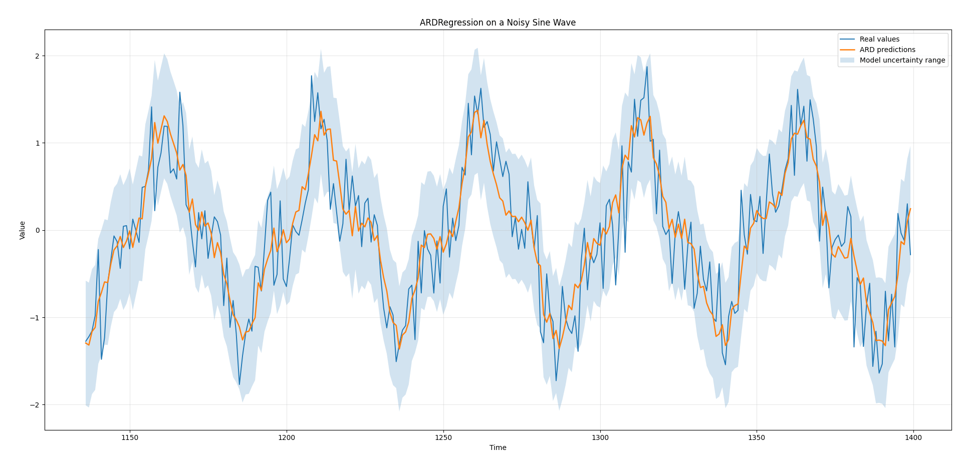
ARD average error: 0.310
Baseline average error: 0.425
ARD large-error score: 0.391
Baseline large-error score: 0.529
Explained share: 0.764
Direction accuracy: 76.136%
Active lags: 49

Most influential lags:
lag_1     0.145027
lag_50    0.073316
lag_65    0.067392
lag_48    0.064639
lag_64    0.059979
lag_23    0.054170
lag_74    0.051897
lag_26    0.050988
lag_29    0.050849
lag_72    0.050070
What the script is doing
The random seed ensures that the same synthetic series is produced each time the script runs.
The clean signal contains two repeating movements. One completes a cycle every 50 observations. The other completes a cycle every 17 observations and has a smaller effect.
Random noise is then added to every observation. The model sees only the noisy result. It does not receive the clean signal, the cycle lengths, or any direct indication that two separate patterns exist.
The lag-building section creates 80 historical inputs. For every usable row, lag_1 contains the immediately previous value, lag_2 contains the value from two periods earlier, and the process continues through lag_80.
The first 80 rows are removed because they do not have a complete history.
The chronological split then places the earlier observations in the training sample and the later observations in the test sample. No shuffling takes place.
The scaler is trained only on the training inputs. It then applies the same transformation to the test inputs.
This ordering matters. Fitting the scaler on the complete dataset would allow information from the test period to influence the preparation of the training data. The leakage would be small in this synthetic example, but the research process should remain correct even when the effect appears harmless.
The model is fitted using up to 1,000 training iterations. It usually stops earlier once its internal estimates become stable.
The prediction step returns two outputs. The first is the predicted value. The second is the model’s uncertainty estimate.
The baseline uses lag_1, meaning that it predicts no change from the most recent observation.
Reading the chart
The real series should appear visibly noisier than the model prediction.
This is expected.
The random disturbance added to every observation cannot be forecast from earlier values. A sensible model should recover the repeating structure without attempting to reproduce every isolated jump.
As a result, the prediction line tends to move through the centre of the noisy observations. It follows the main rises and falls while ignoring some of the sharpest fluctuations.
That smoother appearance does not automatically indicate underfitting. The target contains both predictable structure and unpredictable noise. Reproducing the noise would improve the visual fit on known data but would not provide a dependable forecasting advantage on unseen observations.
The shaded region represents the model’s estimated uncertainty.
It tends to remain fairly stable in this experiment because the test data resembles the training data. The series continues to follow the same general process, with the same cycle structure and noise level.
A more revealing uncertainty experiment would alter the test period by changing the cycle length, increasing the noise, or introducing a trend. The model would then face observations that are less consistent with its training history.
Even then, the uncertainty estimate may not fully recognise the structural change. ARDRegression measures uncertainty within its own learned framework. It does not possess a separate mechanism for detecting every form of regime shift.
Performance evaluation
With the fixed random seed used in the script, the exact output may vary slightly across software versions, but a representative run produces an average model error of approximately 0.310.
The persistence baseline produces an average error of approximately 0.425.
This means the ARD model reduces the average miss by roughly 27 percent relative to simply carrying the latest observation forward.
The score that places greater emphasis on large mistakes is approximately 0.391 for ARDRegression and 0.529 for the baseline. The model therefore improves both typical accuracy and protection against larger misses.
The explained share is approximately 0.764. In practical language, the model captures a substantial portion of the movement in the unseen test period, while the remaining variation includes random noise and modelling error.
The directional accuracy is approximately 76 percent. This measures whether the model correctly predicts whether the next value will rise or fall relative to the most recent observation.
This result should be interpreted carefully.
The synthetic series contains persistent repeating behaviour. Its direction is much easier to predict than the direction of a highly irregular financial return series. The experiment demonstrates that ARDRegression can recover recurring temporal structure from noisy lagged observations. It does not demonstrate that the same directional accuracy should be expected in markets.
The comparison with the baseline is especially important.
A smooth cyclical series naturally gives the most recent observation predictive value. The baseline is therefore not useless. It already follows the series reasonably well.
ARDRegression improves on it because the model can use a wider historical window. It can recognise where the series appears to be within its repeating movement rather than assuming that the current level will persist unchanged.
Interpreting the selected lags
The script reports how many lag inputs remain active and prints the ten with the strongest influence.
The strongest lag will often be the most recent observation. This is reasonable because the series moves continuously and nearby values tend to resemble one another.
Other influential lags may appear near the underlying cycle lengths or at positions that help identify the current phase of the repeating pattern.
The results should not be interpreted too literally.
The two waves overlap, and many neighbouring lags contain similar information. The model does not need to identify the exact cycle lengths in order to forecast effectively. It may combine several historical positions that together describe the current state of the series.
Different noise samples can also change the selected lags. A lag that appears important in one run may lose influence in another.
This is why feature stability should be tested across multiple chronological training windows. A lag that remains influential across many periods is more credible than one that appears only in a single fitted sample.
Scikit-learn’s own comparison examples show that ARDRegression can produce a sparser solution by setting some uninformative inputs to zero, while also noting that some irrelevant inputs may still retain influence. Automatic relevance selection reduces the problem; it does not grant the model supernatural judgment.
Strengths and limitations
Strengths
ARDRegression is useful when the researcher has many candidate inputs but expects only part of them to be genuinely informative.
This situation is common in time-series work. A dataset may contain dozens of lags, several rolling windows, multiple indicators, and related external series. Manually selecting a small subset can be arbitrary, while keeping everything can produce an unstable model.
ARDRegression offers a middle path. The researcher provides a broad candidate set, and the model reduces the role of weak inputs during training.
The resulting model remains relatively interpretable. Each input receives a visible influence value, and inputs removed by the relevance process can be identified.
This is considerably easier to inspect than a large tree ensemble or neural network. A researcher can examine which lags remain active, whether their importance changes over time, and whether the selected structure makes economic or scientific sense.
The model also provides a built-in uncertainty estimate. This is useful when the forecast must be considered alongside an indication of confidence rather than as a single unquestionable value.
ARDRegression can perform well on small and medium-sized datasets. It does not require the enormous training samples often associated with more complex models.
Its automatic restraint can also reduce overfitting when the number of candidate inputs is large relative to the amount of available data.
Limitations
ARDRegression remains a linear model.
It combines inputs through fixed influences. It does not naturally learn rules such as one relationship applying during high volatility and another applying during low volatility.
Nonlinear behaviour must be represented through additional engineered inputs or handled by another model class.
The model also assumes that the relationship learned during training remains reasonably stable during the test period. If the underlying process changes, the selected lags may no longer be relevant.
This matters greatly in financial time series. Market behaviour can change after policy shifts, volatility shocks, structural breaks, or changes in participant behaviour. A model trained on one environment may carry obsolete relationships into another.
Correlated inputs create another interpretive problem.
If several lags contain nearly identical information, the model may distribute influence across them or favour one somewhat arbitrarily. The selected features should not be treated as independent discoveries.
Computation can become expensive when the input set grows very large. ARDRegression performs repeated internal updates and is generally slower than simpler linear methods. Hundreds of features may remain manageable, but thousands of heavily overlapping features can make training less convenient.
The uncertainty range also has limits.
It reflects uncertainty as understood by the fitted model. It does not automatically account for data errors, unprecedented events, sudden regime changes, or incorrect assumptions in the feature design.
Finally, automatic relevance determination does not eliminate the need for careful validation.
A single chronological train-test split is adequate for demonstration, but serious research should repeat the process across multiple forward-moving windows. Performance, selected inputs, and uncertainty behaviour should all be examined through time.
A model that performs well in one final test segment may simply have encountered a favourable period. The more important question is whether it continues to add value across changing samples without relying on future information.