


Applying the Gradient Boost Regressor on Time Series in Python
Presenting and Coding a Machine Learning Model on Time Series


This article will discuss a machine learning model referred to as Gradient Boost Regressor. We will download a time series from an online source, transform it (i.e. make it stationary) and will simply apply the model’s tools to forecast t+1 values at each time step. We will just apply a simple performance evaluation tool, that is the accuracy (or hit ratio).
Intuition of the Model
Gradient Boosting is a powerful ensemble technique that has established itself as a top-performing approach for regression and classification tasks across a wide range of domains. Among its implementations, the GradientBoostingRegressor—as provided in libraries such as scikit-learn—offers a robust, scalable solution for predictive modeling. It builds a strong predictive model by sequentially combining multiple weak learners, typically decision trees, into a single ensemble model.
The model is based on the principle of gradient boosting, an iterative function approximation method. At each iteration, a new model is trained to predict the residual errors (gradients) of the combined ensemble from the previous step. By minimizing a specified loss function, typically the mean squared error for regression, the model incrementally improves prediction accuracy.
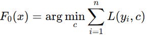
Formally, given a training set (x, y) for i = 1, …, n, the goal is to find a function F(x) that minimizes the expected value of a loss function L(y,F(x)). The model is initialized with a constant prediction:
At each stage m = 1, …, M = 1, the algorithm computes the negative gradient of the loss function with respect to the current prediction:

A base learner h(x), typically a shallow regression tree, is then fit to these residuals. The ensemble is updated as:

where ν ∈ (0,1] is the learning rate that controls the contribution of each tree.
This additive model-building approach allows the regressor to correct errors from previous iterations gradually, reducing bias while controlling variance. The final model is a weighted sum of the base learners:

Key hyperparameters, such as the number of estimators M, learning rate ν, and maximum depth of trees, allow the model to balance bias-variance trade-offs and prevent overfitting.
Do you want to master Deep Learning techniques tailored for time series, trading, and market analysis🔥? My book breaks it all down from basic machine learning to complex multi-period LSTM forecasting while going through concepts such as fractional differentiation and forecasting thresholds. Get your copy here 📖!
Using the Model to Forecast Time Series
Let’s use the model in Python to apply the returns of a time series. We’ll choose the returns of S&P 500 for this task, while knowing that it’s almost impossible to accurately predict such a chaotic dataset with simple models, but we will do it just to make the models work. The plan of attack is as follows:
Download the time series.
Take the returns of the prices to make it stationary (an important condition of machine learning forecasting).
Split the data into training and test sets.
Fit and predict.
Evaluate and plot the predictions.
Use the following code to conduct the experiment.
from sklearn.ensemble import GradientBoostingRegressor
import pandas_datareader as pdr
import numpy as np
import matplotlib.pyplot as plt

def data_preprocessing(data, num_lags, train_test_split):
    # Prepare the data for training
    x = []
    y = []
    for i in range(len(data) - num_lags):
        x.append(data[i:i + num_lags])
        y.append(data[i+ num_lags])
    # Convert the data to numpy arrays
    x = np.array(x)
    y = np.array(y)
    # Split the data into training and testing sets
    split_index = int(train_test_split * len(x))
    x_train = x[:split_index]
    y_train = y[:split_index]
    x_test = x[split_index:]
    y_test = y[split_index:]
    return x_train, y_train, x_test, y_test
start_date = '1960-01-01'
end_date   = '2020-01-01'
# Import the data
data = (pdr.get_data_fred('SP500', start = start_date, end = end_date).dropna())
data = np.diff(data['SP500'])
# Train-test split
x_train, y_train, x_test, y_test = data_preprocessing(data, 100, 0.80)
# Create and train the model
model = GradientBoostingRegressor()
model.fit(x_train, y_train)
# Make predictions on the test set
y_pred = model.predict(x_test)
# Evaluate the model
same_sign_count = np.sum(np.sign(y_pred) == np.sign(y_test)) / len(y_test) * 100
print('Hit Ratio = ', same_sign_count, '%')
# Plot the actual vs. predicted values
plt.figure(figsize=(12, 6))
plt.plot(y_test[-50:], label = 'Actual', color = 'blue')
plt.plot(y_pred[-50:], label = 'Predicted', color = 'red')
plt.legend()
plt.title('Actual vs. Predicted')
plt.ylabel('Value')
plt.show()
plt.grid()
plt.axhline(y = 0, color = 'black')
The following is the plot that compares the real data from the test set and the predicted data.

The following output shows the hit ratio.
44.66%As with any technique out there, the simple versions (default) are just building blocks from where you will improve on them.
Every week, I analyze positioning, sentiment, and market structure. Curious what hedge funds, retail, and smart money are doing each week? Then join hundreds of readers here in the Weekly Market Sentiment Report 📜 and stay ahead of the game through chart forecasts, sentiment analysis, volatility diagnosis, and seasonality charts.
Free trial available🆓
