
A-Z Machine Learning: Random Forest in Time Series Analysis
A Deep Understanding and Visualization of Random Forest


Random Forest is a robust and versatile machine learning technique often used for prediction and classification tasks. Unlike linear regression, which works with a straight line to make predictions, Random Forest is more like a sophisticated ensemble of decision trees.
This article shows you everything you need to know about random forest, and presents a full example of applying it on time series in order to predict the future values.
Intuition of a Decision Tree
Decision trees are a visual representation of a decision-making process, starting with a root node that represents the initial decision. At each node in the tree, a decision or test is made based on a specific feature, and branches represent possible outcomes. The leaves of the tree signify final outcomes or predicted values.
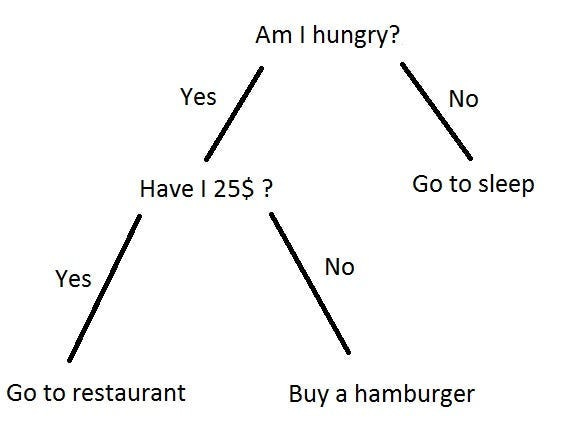
The decision-making process involves splitting nodes based on particular features, like the number of bedrooms in a house price prediction. Various criteria, such as Gini impurity for classification or mean squared error for regression, guide the decision on how to split nodes and determine the importance of features.
Gini impurity quantifies how often a randomly chosen element from the set would be incorrectly labeled if it was randomly labeled according to the distribution of labels in the set. The mean squared error (MSE) quantifies how far off your predictions are from the true values and provides a measure of the model’s accuracy.
During training, decision trees learn from labeled data, adjusting to find the best features and optimal values for splits to minimize impurity or error. To avoid overfitting, where the tree captures noise in the data, pruning can be applied to trim unnecessary branches.
One notable advantage of decision trees is their interpretability — they are easy to understand and explain, making them useful for clarifying decision processes. They can handle both numerical and categorical data, adding to their versatility.
However, decision trees have limitations, including sensitivity to small data changes and a tendency to overfit. To address these issues, ensemble methods like random forests use multiple decision trees to enhance predictive performance.
Decision trees rely on several considerations (as opposed to assumptions) to provide accurate and reliable results. Here are the key assumptions explained in simpler terms:
Non-linearity: Decision trees assume that the relationships between features and outcomes are non-linear. They are well-suited for capturing complex patterns and interactions in the data.
Variable independence: Decision trees assume that features used for decision-making are independent. In reality, this might not always be the case, and the performance of the tree can be affected if there are strong correlations between features.
Sensitive to noisy data: Decision trees can be sensitive to noise in the data. Outliers or small variations in the training data might lead to overfitting, where the tree captures patterns that don’t generalize well to new data.
Overfitting: Overfitting is a concern with decision trees, especially if the tree is deep and captures noise in the training data. Pruning* techniques can be applied to mitigate overfitting.
Limited expressiveness: While decision trees are versatile, they might struggle with problems where the relationships between features and outcomes are too intricate or involve subtle nuances that require more sophisticated models.
Binary splits: Traditional decision trees typically use binary splits, meaning they divide the data into two groups at each node. This might not always capture more complex relationships that involve multiple outcomes.
Handling imbalanced data: Decision trees might not perform well on imbalanced datasets, where one class significantly outnumbers the others. Techniques like adjusting class weights or using ensemble methods can help address this issue.
*Pruning in the context of decision trees refers to the process of removing parts of the tree that do not contribute significantly to its predictive accuracy. The primary goal of pruning is to prevent overfitting, where a tree captures noise or specific patterns in the training data that do not generalize well to new, unseen data.
Check out my newsletter that sends weekly directional views every weekend to highlight the important trading opportunities using a mix between sentiment analysis (COT report, put-call ratio, etc.) and rules-based technical analysis.

Random Forest Algorithm
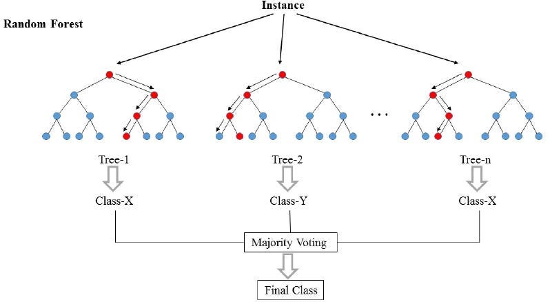
Random forest is an ensemble learning method that builds multiple decision trees during training and merges their predictions to improve overall accuracy and reduce overfitting. Let’s break down it and compare it with individual decision trees.
Random forest builds multiple decision trees independently during the training process. Each tree is trained on a random subset of the data (bootstrap sample) and may consider only a random subset of features at each split. Advantages over Individual Decision Trees:
Improved accuracy: Random Forest often provides higher accuracy compared to a single decision tree, especially on complex datasets.
Handle more features: It can handle a larger number of features and capture complex relationships by combining the strengths of multiple trees.
Less prone to overfitting: The ensemble nature of Random Forest makes it less prone to overfitting, enhancing its generalization to new data.
Evaluating a Random Forest Model
There are many ways to evaluate the random forest model. If you are interested in a binary directional model (such as positive change and negative change), then you can add accuracy as a performance criteria. We will see how the binary model works.
Here are some other ways you can evaluate the model:
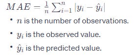
Mean absolute error (MAE): Average of the absolute differences between predicted and observed values. Lower values are better.
Mean squared error (MSE): Average of the squared differences between predicted and observed values. Commonly used but sensitive to outliers.

Root mean squared error (RMSE): Square root of MSE. Provides a measure in the same units as the dependent variable. Like MSE, sensitive to outliers.

Mean absolute percentage error (MAPE): Average of the percentage differences between predicted and observed values. Useful when dealing with relative errors.

A Practical Python Example
Imagine you’re trying to make predictions, like predicting the price of a house. Instead of relying on a single decision tree, which might be too simplistic, Random forest combines the power of multiple trees. Each tree in the forest makes its own prediction, and then they “vote” to decide the final outcome. It’s like having a committee of experts sharing their opinions, and the collective wisdom tends to be more accurate and resilient than relying on just one perspective.
Random forest is great for handling complex relationships between input features and outputs. It can capture non-linear patterns and interactions, making it particularly useful in situations where a linear approach might fall short.
While it might seem more complex than linear regression, its strength lies in its ability to handle intricate data patterns and make more accurate predictions, even in the world of finance, where complex relationships often exist.
Now, let’s take a time series example and try to forecast its future values. This time series will be the Bitcoin fear and greed index.
The Bitcoin fear and greed index is a tool that attempts to gauge the sentiment of the market towards Bitcoin. It ranges from 0 to 100 and is calculated based on various factors such as price volatility, trading volume, social media sentiment, and surveys.
When the index is high, like 80 or above, it indicates extreme greed in the market. This means investors might be too optimistic, and there’s a possibility of a correction. On the other hand, a low index, say 20 or below, suggests extreme fear, signaling that investors might be overly pessimistic, and there could be opportunities for buying.
It’s essential to note that the index is just one tool among many, and relying solely on it might not provide a comprehensive view of the market. It’s always wise to consider various indicators and do thorough research before making any financial decisions, especially in the volatile world of cryptocurrencies.
The plan of attack is as follows:
Download the index data from this GitHub repository and upload it to Python.
Take the differences of the index data. It is already stationary, but we do this to measure the directional accuracy.
Split the data into a training set and a test set.
Fit the model using the last index change (thus, binary) as features. Then, predict on never-seen-before data in the test set.
Evaluate and compare the predicted versus real data.
Use the following code to implement the process (make sure to download the fear and greed index data from the repository):
import numpy as np
from sklearn.ensemble import RandomForestRegressor
import matplotlib.pyplot as plt
import pandas as pd

def data_preprocessing(data, num_lags, train_test_split):
    # Prepare the data for training
    x = []
    y = []
    for i in range(len(data) - num_lags):
        x.append(data[i:i + num_lags])
        y.append(data[i+ num_lags])
    # Convert the data to numpy arrays
    x = np.array(x)
    y = np.array(y)
    # Split the data into training and testing sets
    split_index = int(train_test_split * len(x))
    x_train = x[:split_index]
    y_train = y[:split_index]
    x_test = x[split_index:]
    y_test = y[split_index:]

    return x_train, y_train, x_test, y_test
# Import data
data = pd.read_excel('Fear_Greed_BTCUSD.xlsx').values
data = np.reshape(data, (-1))
data = np.diff(data)
x_train, y_train, x_test, y_test = data_preprocessing(data, 1, 0.90)
# Create a Regressor model
model = RandomForestRegressor(max_depth = 100, random_state = 123)
# Fit the model to the data
model.fit(x_train, y_train)
# Predict on the same data used for training
y_pred = model.predict(x_test)
# Plotting
plt.plot(y_pred[-50:], label='Predicted Data', linestyle='--', marker = '.')
plt.plot(y_test[-50:], label='True Data', marker = '.')
plt.legend()
plt.grid()
plt.axhline(y = 0, color = 'black', linestyle = '--')
import math
from sklearn.metrics import mean_squared_error
rmse_test = math.sqrt(mean_squared_error(y_pred, y_test))
print(f"RMSE of Test: {rmse_test}")
same_sign_count = np.sum(np.sign(y_pred) == np.sign(y_test)) / len(y_test) * 100
print('Directional Accuracy = ', same_sign_count, '%')
The output of the code is as follows:
RMSE of Test: 3.87
Directional Accuracy =  54.28 %
It seems that with a directional accuracy of 54.28%, the model is able to predict whether there will be a positive or a negative change from the last change. The RMSE shows that the forecasts have an error term of around 3.87. This leaves much room for improvement.
Improvement can be in the sense of adding more features, changing the number of lagged inputs, and adding any other conditions.