A New Variation on the Bollinger Bands in Python.
Coding an Bands Indicator Using the Volatility-Adjusted Moving Average.
The great Bollinger Bands are one of the first things we must learn when analyzing time series. This is because of their sound statistical reasoning, their wide adoption across market participants, and their success when deployed in trading strategies. We can also see other variations that resemble the Bands in an attempt to enhance it.
I have just published a new book after the success of my previous one “New Technical Indicators in Python”. It features a more complete description and addition of structured trading strategies with a GitHub page dedicated to the continuously updated code. If you feel that this interests you, feel free to visit the below link, or if you prefer to buy the PDF version, you could contact me on LinkedIn.
The Volatility-Adjusted Moving Average
In a previous article, we have introduced the Volatility-Adjusted Moving Average — VAMA — created by Tushar Chande. This part is a continuation towards creating volatility bands around them to create dynamic support nd resistance levels. First, w refresher on the VAMA before moving on.
The volatility-adjusted moving average — VAMA — is a technical indicator created by Tushar S. Chande. Commonly referred to as the Variable Index Moving Average, it is a powerful indicator that uses two standard deviation periods to account for recent volatility. I have taken the liberty to rename it into the volatility-adjusted moving average because there is a newer version with the same name that uses the Chande momentum oscillator instead of the standard deviation, hence it is important to distinguish the difference between the two.
The first step to calculate the VAMA is to measure the alpha which can be found through this formula below:
Therefore, the alpha is calculated as a ratio between a short-term volatility calculation and a long-term volatility calculation. The result is multiplied by 0.20. Then, to calculate the VAMA, we follow these steps.
The first VAMA value is simply the closing price, and then the algorithm can take the form of the above formula.
The above chart shows the EURUSD hourly values with the VAMA using a 3-period standard deviation and a 144-period standard deviation. To code the VAMA, we use the below function
# The function to add a number of columns inside an array
def adder(Data, times):

    for i in range(1, times + 1):

        new_col = np.zeros((len(Data), 1), dtype = float)
        Data = np.append(Data, new_col, axis = 1)

    return Data
# The function to delete a number of columns starting from an index
def deleter(Data, index, times):
for i in range(1, times + 1):
Data = np.delete(Data, index, axis = 1)
return Data
# The function to delete a number of rows from the beginning
def jump(Data, jump):
Data = Data[jump:, ]
return Data# Example of adding 3 empty columns to an array
my_ohlc_array = adder(my_ohlc_array, 3)# Example of deleting the 2 columns after the column indexed at 3
my_ohlc_array = deleter(my_ohlc_array, 3, 2)# Example of deleting the first 20 rows
my_ohlc_array = jump(my_ohlc_array, 20)# Remember, OHLC is an abbreviation of Open, High, Low, and Close and it refers to the standard historical data filedef volatility(Data, lookback, what, where):
# Adding an extra column
Data = adder(Data, 1)
for i in range(len(Data)):
try:
Data[i, where] = (Data[i - lookback + 1:i + 1, what].std())
except IndexError:
pass
# Cleaning
Data = jump(Data, lookback)
return Datadef ma(Data, lookback, close, where):
Data = adder(Data, 1)
for i in range(len(Data)):
try:
Data[i, where] = (Data[i - lookback + 1:i + 1, close].mean())
except IndexError:
pass
# Cleaning
Data = jump(Data, lookback)
return Datadef volatility_adjusted_moving_average(Data, lookback_volatility_short, lookback_volatility_long, close, where):
# Adding Columns
Data = adder(Data, 2)
# Calculating Standard Deviations
Data = volatility(Data, lookback_volatility_short, close, where)
Data = volatility(Data, lookback_volatility_long, close, where + 1)
# Calculating Alpha
for i in range(len(Data)):
Data[i, where + 2] = 0.2 * (Data[i, where] / Data[i, where + 1])
# Calculating the First Value of VAMA
Data[1, where + 3] = (Data[1, where + 2] * Data[1, close]) + ((1 - Data[1, where + 2]) * Data[0, close])
# Calculating the Rest of VAMA
for i in range(2, len(Data)):
Data[i, where + 3] = (Data[i, where + 2] * Data[i, close]) + ((1 - Data[i, where + 2]) * Data[i - 1, where + 3]) # Cleaning
Data = deleter(Data, where, 3)
Data = jump(Data, 1)
return Datalookback_volatility_short = 3
lookback_volatility_long = 144my_data = volatility_adjusted_moving_average(my_data, lookback_volatility_short, lookback_volatility_long, 3, 4)The way to use the VAMA is to follow the trend with it or simply expect reactions from it whenever the market approaches it. There are a lot of combinations to be made with this moving average like what we will do in the next section.
The VAMA Bands
Volatility bands try to envelop the prices using mathematical techniques. The main aim is to find statistical extremes that act as support and resistance levels in ranging markets. Even though, it is widely accepted that volatility bands (Such as the Bollinger Bands) are not useful in trending markets, their utility has stood the test of time. This section will simply apply the formula of the volatility bands using the VAMA.
We will calculate a rolling 30-period standard deviation on the price.
We will multiply the standard deviation of each time step (Row) by 3.
We will add it to the current VAMA to find a dynamic resistance level.
We will subtract it from the current VAMA to find a dynamic support level.
def vama_bands(Data, lookback_volatility_short, lookback_volatility_long, lookback_volatility, std, close, where):

    Data = volatility_adjusted_moving_average(Data, lookback_volatility_short, lookback_volatility_long, close, where)

    Data = volatility(Data, lookback_volatility, close, where + 1)

    Data = adder(Data, 2)

    Data[:, where + 2] = Data[:, where] + (std * Data[:, where + 1])
    Data[:, where + 3] = Data[:, where] - (std * Data[:, where + 1])

    Data = jump(Data, lookback_volatility)
    Data = deleter(Data, where + 1, 1)

    return Data
lookback_volatility_short = 3
lookback_volatility_long = 144
lookback_volatility = 30
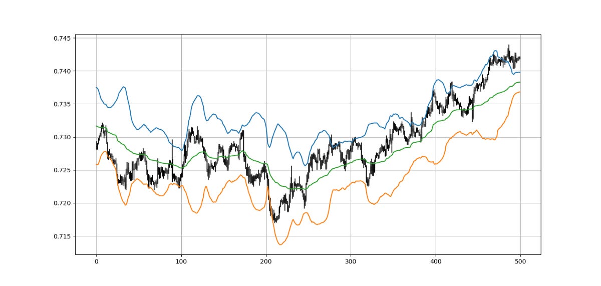
std = 3my_data = vama_bands(my_data, lookback_volatility_short, lookback_volatility_long, lookback_volatility, std, 3, 4)The above chart shows the hourly values of the AUDUSD with a VAMA in green that uses 3 periods for the short standard deviation and 144 periods for the long standard deviation. Also plotted are the bands that use a rolling 30 periods for standard deviation and a multiplier of 3.
def signal(Data, close, upper_boll, lower_boll, buy, sell):

    Data = adder(Data, 10)

    for i in range(len(Data)):

        if Data[i, close] < Data[i, lower_boll] and Data[i - 1, close] > Data[i - 1, lower_boll]:

            Data[i, buy] = 1

        if  Data[i, close] > Data[i, upper_boll] and Data[i - 1, close] < Data[i - 1, upper_boll]:

            Data[i, sell] = -1

    return Data
If you are also interested by more technical indicators and using Python to create strategies, then my best-selling book on Technical Indicators may interest you:
Conclusion
Remember to always do your back-tests. You should always believe that other people are wrong. My indicators and style of trading may work for me but maybe not for you.
I am a firm believer of not spoon-feeding. I have learnt by doing and not by copying. You should get the idea, the function, the intuition, the conditions of the strategy, and then elaborate (an even better) one yourself so that you back-test and improve it before deciding to take it live or to eliminate it. My choice of not providing specific Back-testing results should lead the reader to explore more herself the strategy and work on it more.
To sum up, are the strategies I provide realistic? Yes, but only by optimizing the environment (robust algorithm, low costs, honest broker, proper risk management, and order management). Are the strategies provided only for the sole use of trading? No, it is to stimulate brainstorming and getting more trading ideas as we are all sick of hearing about an oversold RSI as a reason to go short or a resistance being surpassed as a reason to go long. I am trying to introduce a new field called Objective Technical Analysis where we use hard data to judge our techniques rather than rely on outdated classical methods.


