A Moving Average Crossover Strategy With the Same Lookback Period

Creating a Moving Average Crossover Strategy With One Lookback Period

Generally, when we think about a moving average crossover strategy, we think about two different moving averages with different lookback periods so that it makes sense. This article presents a way of removing that subjective choice and performing the strategy with just one lookback period.

I have released a new book after the success of my previous one “Trend Following Strategies in Python”. It features advanced contrarian indicators and strategies with a GitHub page dedicated to the continuously updated code. If you feel that this interests you, feel free to visit the below Amazon link (which contains a sample), or if you prefer to buy the PDF version, you could check the link at the end of the article.

Contrarian Trading Strategies in Python
Amazon.com: Contrarian Trading Strategies in Python: 9798434008075: Kaabar, Sofien: Bookswww.amazon.com

---

A Primer on Weighted Moving Averages

The way we will design our same-lookback crossover strategy will be by using weighted moving averages.

A weighted moving average is a simple moving average that places more weight on recent data. The most recent observation has the biggest weight and each one prior to it has a progressively decreasing weight. Structurally, it has less lag than the other moving averages but it is also the least used, and hence, what it gains in lag reduction, it loses in popularity. Mathematically speaking, it can be written down as:

Basically, if we have a dataset composed of two numbers [1, 2] and we want to calculate a linear weighted average, then we will do the following:

• (2 x 2) + (1 x 1) = 5

• 5 / 3 = 1.66

Now, what if we invert this reasoning and say that we are interested to place more weight in the most distant data as opposed to the most recent one?

This would mean that we will create an inverse-weighted moving average that shares the same structure as the weighted moving average but with an inverted matrix to be multiplied by the different prices.

Let’s first define the needed libraries needed to create these two moving averages.

import numpy as np

Now, let’s check out the following function that outputs either the weighted or the inverse-weighted moving average depending on what you choose as arguments:

def lwma(data, lookback, type_of_ma = 'weighted'):
    
    weighted = []
    
    for i in range(len(data)):
        
            try:
                
                if type_of_ma == 'inverse-weighted':
                    
                    total = np.arange(lookback, 0, -1)
                    
                elif type_of_ma == 'weighted':  
                    
                    total = np.arange(1, lookback + 1, 1)
                
                matrix = data[i - lookback + 1: i + 1, 3:4]
                matrix = np.ndarray.flatten(matrix)
                matrix = total * matrix
                
                wma = (matrix.sum()) / (total.sum())
                
                weighted = np.append(weighted, wma)   
       
            except ValueError:
                
                pass
    
    data = data[lookback - 1:, ]
    
    weighted = np.reshape(weighted, (-1, 1)) 
    
    data = np.concatenate((data, weighted), axis = 1)   
    
    return data

The function needs an OHLC array to be applied on. It will create a new column and attach it to the OHLC data. You have already seen how to import data in previous articles.

# To calculate a 100-period weighted moving average
my_data = lwma(my_data, 100, type_of_ma = 'weighted')

# To calculate a 100-period inverse-weighted moving average
my_data = lwma(my_data, 100, type_of_ma = 'inverse-weighted')

---

Creating the Same Lookback Period Moving Average Strategy

A regular moving average crossover strategy requires two moving averages of different lookback periods. For example, one of the most known crossover strategies is between a 60-period moving average and a 200-period moving average. The trading conditions for this type of strategies is as follows:

• A long (buy) signal is generated whenever the short-term moving average (e.g. 60) crosses above the long-term moving average (e.g. 200).

• A short (sell) signal is generated whenever the short-term moving average (e.g. 60) crosses below the long-term moving average (e.g. 200).

In our case, we have created two weighted moving averages of the same lookback period, let’s say 50. Our trading conditions are as follows:

• A long (buy) signal is generated whenever the weighted moving average crosses above the inverse-weighted moving average.

• A short (sell) signal is generated whenever the weighted moving average crosses below the inverse-weighted moving average.

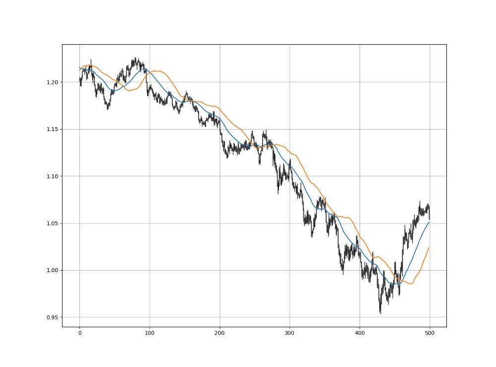
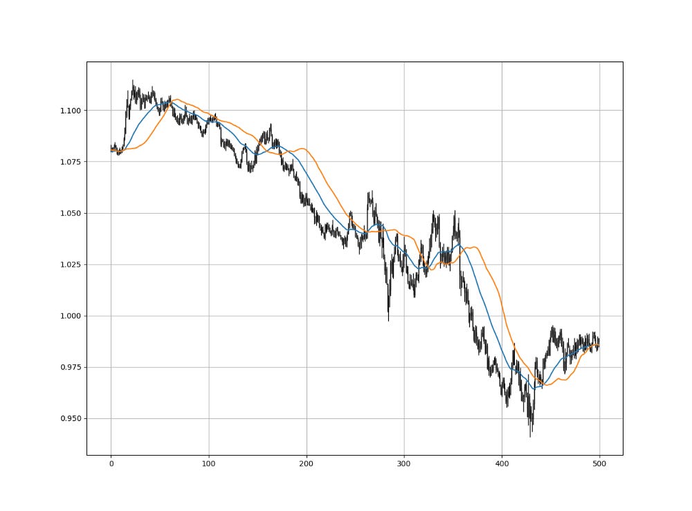
The following Figure shows the two moving averages.

A 50-period weighted moving average in blue and a 50-period inverse-weighted moving average in orange

Clearly, when the weighted moving average (fast) crosses above the inverse-weighted moving average (slow), the market has shaped a push-up or is in the midst of a push-up. In parallel, when the weighted moving average (fast) crosses below the inverse-weighted moving average (slow), the market has shaped a push-down or is in the midst of a push-down.

A 50-period weighted moving average in blue and a 50-period inverse-weighted moving average in orange

This crossover strategy removes the subjective choice of finding the optimal combination of lookback periods. You only need one instead of two.

Getting healthier means changing your lifestyle. Noom Weight helps users lose weight in a sustainable way through behavioral change psychology. It's a no-brainer.